Many of us have encountered incomprehensible terms in various sciences. But there are very few people who are not afraid unclear words, but on the contrary, they encourage and force you to delve deeper into the subject being studied. Today we will talk about such a thing as interpolation. This is a method of constructing graphs using known points, allowing, with a minimum amount of information about a function, to predict its behavior on specific sections of the curve.

Before moving on to the essence of the definition itself and talking about it in more detail, let’s delve a little deeper into history.

Story

Interpolation has been known since ancient times. However, this phenomenon owes its development to several of the most outstanding mathematicians of the past: Newton, Leibniz and Gregory. It was they who developed this concept using more advanced mathematical methods available at that time. Before this, interpolation, of course, was applied and used in calculations, but this was done in completely inaccurate ways that required large quantity data to build a model more or less close to reality.

Today we can even choose which interpolation method is more suitable. Everything is translated into a computer language that can predict the behavior of a function on certain area, limited to known points.

Interpolation is a rather narrow concept, so its history is not so rich in facts. In the next section, we'll figure out what interpolation actually is and how it differs from its opposite - extrapolation.

What is interpolation?

As we have already said, this is the general name for methods that allow you to build a graph by points. In school, this is mainly done by drawing up a table, identifying points on a graph and roughly drawing lines connecting them. The last action is done based on considerations of the similarity of the function under study to others, the type of graphs of which is known to us.

However, there are other, more complex and accurate ways to accomplish the task of plotting a point-by-point graph. So, interpolation is actually a “prediction” of the behavior of a function in a specific area limited by known points.

There is a similar concept associated with the same area - extrapolation. It also represents a prediction of the graph of a function, but beyond the known points of the graph. With this method, a prediction is made based on the behavior of a function over a known interval, and then this function is applied to the unknown interval. This method is very convenient for practical application and is actively used, for example, in economics to predict ups and downs in the market and to predict the demographic situation in the country.

But we have moved away from the main topic. In the next section, we will figure out what interpolation happens and what formulas can be used to perform this operation.

Types of interpolation

The most simple view is interpolation using the nearest neighbor method. Using this method, we get a very rough graph consisting of rectangles. If you have ever seen an explanation of the geometric meaning of an integral on a graph, you will understand what kind of graphical form we are talking about.

In addition, there are other interpolation methods. The most famous and popular are related to polynomials. They are more accurate and allow you to predict the behavior of a function with a fairly meager set of values. The first interpolation method we'll look at is linear polynomial interpolation. This is the simplest method in this category, and probably each of you used it at school. Its essence is to construct straight lines between known points. As you know, a single straight line passes through two points on a plane, the equation of which can be found based on the coordinates of these points. Having constructed these straight lines, we get a broken graph, which at the very least, but reflects the approximate values of the functions and in general outline matches reality. This is how linear interpolation is carried out.

Advanced types of interpolation

There is a more interesting, but also more complex way of interpolation. It was invented by the French mathematician Joseph Louis Lagrange. That is why the calculation of interpolation using this method is named after it: interpolation using the Lagrange method. The trick here is this: if the method outlined in the previous paragraph uses only a linear function for calculation, then the expansion by the Lagrange method also involves the use of polynomials of higher degrees. But it is not so easy to find the interpolation formulas themselves for different functions. And the more points are known, the more accurate the interpolation formula is. But there are many other methods.

There is a more advanced calculation method that is closer to reality. The interpolation formula used in it is a set of polynomials, the application of each of which depends on the section of the function. This method is called a spline function. In addition, there are also ways to do such a thing as interpolate functions of two variables. There are only two methods. Among them are bilinear or double interpolation. This method allows you to easily build a graph using points in three-dimensional space. We will not touch on other methods. In general, interpolation is a universal name for all these methods of constructing graphs, but the variety of ways in which this action can be carried out forces us to divide them into groups depending on the type of function that is subject to this action. That is, interpolation, an example of which we looked at above, refers to direct methods. There is also inverse interpolation, which differs in that it allows you to calculate not a direct, but an inverse function (that is, x from y). We will not consider the latter options, since it is quite complicated and requires a good mathematical knowledge base.

Let's move on to perhaps one of the most important sections. From it we learn how and where the set of methods we are discussing is applied in life.

Application

Mathematics, as we know, is the queen of sciences. Therefore, even if at first you do not see the point in certain operations, this does not mean that they are useless. For example, it seems that interpolation is a useless thing, with the help of which only graphs can be built, which few people need now. However, for any calculations in technology, physics and many other sciences (for example, biology), it is extremely important to present a fairly complete picture of the phenomenon, while having a certain set of values. The values themselves, scattered across the graph, do not always give a clear idea of the behavior of the function in a specific area, the values of its derivatives and points of intersection with the axes. And this is very important for many areas of our lives.

How will this be useful in life?

A question like this can be very difficult to answer. But the answer is simple: no way. This knowledge will not be of any use to you. But if you understand this material and the methods by which these actions are carried out, you will train your logic, which will be very useful in life. The main thing is not the knowledge itself, but the skills that a person acquires in the process of studying. It’s not for nothing that there is a saying: “Live forever, learn forever.”

Related Concepts

You can understand for yourself how important this area of mathematics was (and still is) by looking at the variety of other concepts associated with it. We have already talked about extrapolation, but there is also approximation. Maybe you've already heard this word. In any case, we also discussed what it means in this article. Approximation, like interpolation, are concepts related to the construction of graphs of functions. But the difference between the first and the second is that it is an approximate construction of a graph based on similar known graphs. These two concepts are very similar to each other, which makes it all the more interesting to study each of them.

Conclusion

Mathematics is not as complicated a science as it seems at first glance. She's rather interesting. And in this article we tried to prove it to you. We looked at concepts related to plotting, learned what double interpolation is, and looked at examples where it is used.

There is a situation when in an array known values we need to find intermediate results. In mathematics this is called interpolation. In Excel, this method can be used both for tabular data and for plotting graphs. Let's look at each of these methods.

The main condition under which interpolation can be used is that the desired value must be inside the data array and not outside its limit. For example, if we have a set of arguments 15, 21, and 29, then we can use interpolation to find the function for argument 25. But there is no longer any way to find the corresponding value for argument 30. This is the main difference between this procedure and extrapolation.

Method 1: Interpolation for Tabular Data

First of all, let's look at the applications of interpolation for data that is located in a table. For example, let's take an array of arguments and their corresponding function values, the relationship of which can be described linear equation. This data is shown in the table below. We need to find the corresponding function for the argument 28 . The easiest way to do this is using the operator PREDICTION.

Method 2: Interpolate the graph using its settings

The interpolation procedure can also be used when constructing function graphs. It is relevant if the table on which the graph is based does not indicate the corresponding function value for one of the arguments, as in the image below.

As you can see, the graph has been corrected, and the gap has been removed using interpolation.

Method 3: Interpolate the graph using a function

You can also interpolate the graph using the special ND function. It returns undefined values in the specified cell.

You can do it even easier without running Function Wizard, and just use the keyboard to enter the value into an empty cell "#N/A" without quotes. But it depends on what is more convenient for which user.

As you can see, in Excel you can interpolate as tabular data using the function PREDICTION, and graphics. In the latter case, this can be done using the chart settings or using the function ND causing an error "#N/A". The choice of which method to use depends on the problem statement, as well as the personal preferences of the user.

There are cases when you need to know the results of a function calculation outside the known area. This issue is especially relevant for the forecasting procedure. In Excel there are several ways in which you can perform this operation. Let's look at them with specific examples.

Method 2: Extrapolation for graph

You can perform an extrapolation procedure for a graph by plotting a trend line.

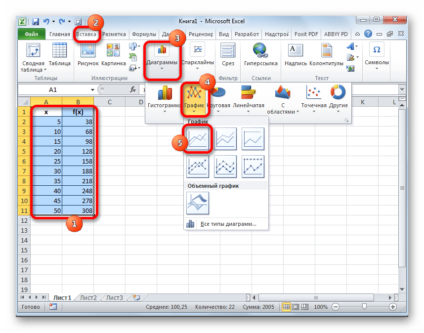
First of all, we build the chart itself. To do this, use the cursor while holding down the left mouse button to select the entire area of the table, including the arguments and corresponding function values. Then, moving to the tab "Insert", click on the button "Schedule". This icon is located in the block "Diagrams" on the tool belt. A list appears available options graphs. We choose the most suitable one at our discretion.

After the graph is constructed, remove the additional argument line from it by selecting it and clicking on the button Delete on the computer keyboard.

Next, we need to change the divisions of the horizontal scale, since it does not display the values of the arguments as we need. To do this, right-click on the diagram and in the list that appears, select the value "Select data".

In the data source selection window that opens, click on the button "Change" in the horizontal axis label editing block.

The window for setting the axis signature opens. Place the cursor in the field of this window, and then select all the data in the column "X" without its name. Then click on the button "OK".

After returning to the data source selection window, we repeat the same procedure, that is, click on the button "OK".

Now our chart is prepared and we can directly begin to build a trend line. Click on the chart, after which an additional set of tabs will be activated on the ribbon - "Working with diagrams". Moving to the tab "Layout" and press the button "Trend line" in the block "Analysis". Click on the item "Linear approximation" or "Exponential Approximation".

The trend line has been added, but it is completely below the line of the graph itself, since we have not specified the value of the argument to which it should tend. To do this, click on the button again. "Trend line", but now select the item "Advanced Trendline Options".

The trendline format window opens. In chapter "Trend Line Options" there is a settings block "Forecast". As in the previous method, let's take the argument for extrapolation 55 . As we can see, so far the graph has a length up to the argument 50 inclusive. It turns out that we will need to extend it for another 5 units. On the horizontal axis you can see that 5 units equals one division. So this is one period. In field "Forward on" enter the value "1". Click on the button "Close" in the lower right corner of the window.

As you can see, the chart has been extended by the specified length using the trend line.

So, we have looked at the simplest examples of extrapolation for tables and graphs. In the first case, the function is used PREDICTION, and in the second - the trend line. But based on these examples, you can decide much more complex tasks forecasting.

Interpolation. Introduction. General statement of the problem

When solving various practical problems, the research results are presented in the form of tables displaying the dependence of one or more measured quantities on one defining parameter (argument). These kinds of tables are usually presented in the form of two or more rows (columns) and are used to form mathematical models.

Tabularly specified in mathematical models functions are usually written in tables of the form:


Y1(X)	Y(X0)	Y(X1)	Y(Xn)

Ym(X)	Y(X0)	Y(X1)	Y(Xn)

The limited information provided by such tables in some cases requires obtaining the values of the functions Y j (X) (j=1,2,…,m) at points X that do not coincide with the nodal points of table X i (i=0,1,2,… ,n) . In such cases, it is necessary to determine some analytical expression φ j (X) to calculate approximate values of the function under study Y j (X) at arbitrarily specified points X. The function φ j (X) used to determine the approximate values of the function Y j (X) is called an approximating function (from the Latin approximo - approaching). The proximity of the approximating function φ j (X) to the approximated function Y j (X) is ensured by choosing the appropriate approximation algorithm.

We will make all further considerations and conclusions for tables containing the initial data of one function under study (i.e. for tables with m=1).

1. Interpolation methods

1.1 Statement of the interpolation problem

Most often, to determine the function φ(X), a formulation is used, called the formulation of the interpolation problem.

In this classical formulation of the interpolation problem, it is required to determine the approximate analytical function φ(X), the values of which at the nodal points X i match the values Y(X i) of the original table, i.e. conditions

ϕ (X i )= Y i (i = 0,1,2,...,n)

The approximating function φ(X) constructed in this way allows one to obtain a fairly close approximation to the interpolated function Y(X) within the range of values of the argument [X 0 ; X n ], determined by the table. When specifying the values of the argument X, not belonging this interval, the interpolation problem is transformed into an extrapolation problem. In these cases, the accuracy

values obtained when calculating the values of the function φ(X) depends on the distance of the value of the argument X from X 0, if X<Х 0 , или отХ n , еслиХ >Xn.

At mathematical modeling the interpolating function can be used to calculate approximate values of the function under study at intermediate points of the subintervals [Х i ; X i+1 ]. This procedure is called table compaction.

The interpolation algorithm is determined by the method of calculating the values of the function φ(X). The simplest and most obvious option for implementing the interpolating function is to replace the function under study Y(X) on the interval [X i ; X i+1 ] by a straight line connecting points Y i , Y i+1 . This method is called the linear interpolation method.

1.2 Linear interpolation

With linear interpolation, the value of the function at point X, located between nodes X i and X i+1, is determined by the formula of a straight line connecting two adjacent points of the table

Y(X) = Y(Xi )+	Y(Xi + 1 )− Y(Xi )	(X − Xi ) (i= 0,1,2, ...,n),

	X i+ 1− X i

In Fig. Figure 1 shows an example of a table obtained as a result of measurements of a certain quantity Y(X). The rows of the source table are highlighted. To the right of the table is a scatter plot corresponding to this table. The table is compacted using the formula

(3) values of the approximated function at points X corresponding to the midpoints of the subintervals (i=0, 1, 2, …, n).

Fig.1. Condensed table of the function Y(X) and its corresponding diagram

When considering the graph in Fig. 1 it can be seen that the points obtained as a result of compacting the table using the linear interpolation method lie on straight segments connecting the points of the original table. Linear accuracy

interpolation, significantly depends on the nature of the interpolated function and on the distance between the nodes of the table X i, , X i+1.

Obviously, if the function is smooth, then, even with relatively long distance between nodes, a graph constructed by connecting points with straight line segments allows one to fairly accurately assess the nature of the function Y(X). If the function changes quite quickly, and the distances between the nodes are large, then the linear interpolating function does not allow obtaining a sufficiently accurate approximation to the real function.

The linear interpolating function can be used for general preliminary analysis and assessment of the correctness of interpolation results, which are then obtained by other more accurate methods. This assessment becomes especially relevant in cases where calculations are performed manually.

1.3 Interpolation by canonical polynomial

The method of interpolating a function by a canonical polynomial is based on constructing the interpolating function as a polynomial in the form [1]

ϕ (x) = Pn (x) = c0 + c1 x+ c2 x2 + ... + cn xn

Coefficients c i of polynomial (4) are free interpolation parameters, which are determined from Lagrange conditions:

Pn (xi )= Yi , (i= 0 , 1 , ... , n)

Using (4) and (5) we write the system of equations

C x+ c x2		C xn = Y

C x+ c x2		C xn


	C x2		C xn = Y

The solution vector with i (i = 0, 1, 2, …, n) of the system of linear algebraic equations (6) exists and can be found if there are no matching nodes among i. The determinant of system (6) is called the Vandermonde determinant1 and has an analytical expression [2].

1 Vandermonde determinant called determinant

It is equal to zero if and only if xi = xj for some. (Material from Wikipedia - the free encyclopedia)

To determine the values of coefficients with i (i = 0, 1, 2, … , n)

equations (5) can be written in vector-matrix form

A* C= Y,

where A, matrix of coefficients determined by the table of degrees of the vector of arguments X = (x i 0, x i, x i 2, …, x i n) T (i = 0, 1, 2, …, n)

				x0 2		x0 n




				xn 2		xn n

C is the column vector of coefficients i (i = 0, 1, 2, … , n), and Y is the column vector of values Y i (i = 0, 1, 2, … , n) of the interpolated function at the interpolation nodes.

The solution to this system of linear algebraic equations can be obtained using one of the methods described in [3]. For example, according to the formula


C = A− 1 Y,

where A -1 is the inverse matrix of matrix A. To obtain the inverse matrix A -1, you can use the MOBR() function included in the set standard features programs Microsoft Excel.

After the values of the coefficients with i are determined using function (4), the values of the interpolated function can be calculated for any value of the arguments.

Let's write matrix A for the table shown in Fig. 1, without taking into account the rows that compact the table.

Fig.2 Matrix of the system of equations for calculating the coefficients of the canonical polynomial

Using the MOBR() function, we obtain matrix A -1 inverse to matrix A (Fig. 3). After which, according to formula (9) we obtain the vector of coefficients C = (c 0 , c 1 , c 2 , …, c n ) T shown in Fig. 4.

To calculate the values of the canonical polynomial in the cell of the Y canonical column corresponding to the values x 0, we introduce a formula converted to the following form, corresponding to the zero row of system (6)

=((((c 5	* x 0 +c 4 )x 0 +c 3 )x 0 +c 2 )x 0 +c 1 )x 0 +c 0

C0 +x *(c1 + x *(c2 + x*(c3 + x*(c4 + x* c5 ))))

Instead of writing " c i " in the formula entered into an Excel table cell, there should be an absolute link to the corresponding cell containing this coefficient (see Fig. 4). Instead of "x 0" - a relative reference to a cell in column X (see Fig. 5).

Y canonical(0) of the value that matches the value in cell Ylin(0) . When stretching the formula written into cell Y canonical (0), the values of Y canonical (i) corresponding to the nodal points of the original must also coincide

tables (see Fig. 5).

Rice. 5. Diagrams built using linear and canonical interpolation tables

Comparing the graphs of functions constructed from tables calculated using linear and canonical interpolation formulas, we see in a number of intermediate nodes a significant deviation of the values obtained using linear and canonical interpolation formulas. A more reasonable judgment on the accuracy of interpolation can be based on obtaining additional information about the nature of the modeled process.

This is a chapter from Bill Jelen's book.

Challenge: Some engineering design problems require the use of tables to calculate parameter values. Since the tables are discrete, the designer uses linear interpolation to obtain an intermediate parameter value. The table (Fig. 1) includes height above the ground (control parameter) and wind speed (calculated parameter). For example, if you need to find the wind speed corresponding to a height of 47 meters, then you should apply the formula: 130 + (180 – 130) * 7 / (50 – 40) = 165 m/sec.

Download the note in or format, examples in format

What if there are two control parameters? Is it possible to perform calculations using one formula? The table (Fig. 2) shows the wind pressure values for various heights and span sizes of structures. It is required to calculate the wind pressure at a height of 25 meters and a span of 300 meters.

Solution: We solve the problem by extending the method used for the case with one control parameter. Follow these steps:

Start with the table shown in Fig. 2. Add source cells for height and span in J1 and J2 respectively (Figure 3).

Rice. 3. Formulas in cells J3:J17 explain the operation of the megaformula

For ease of use of formulas, define names (Fig. 4).

Watch the formula work sequentially from cell J3 to cell J17.

Use reverse sequential substitution to construct the megaformula. Copy the formula text from cell J17 to J19. Replace the reference to J15 in the formula with the value in cell J15: J7+(J8-J7)*J11/J13. And so on. The result is a formula consisting of 984 characters, which cannot be perceived in this form. You can look at it in the attached Excel file. I'm not sure that this kind of megaformula is useful to use.

Summary: Linear interpolation is used to obtain an intermediate parameter value if table values are specified only for range boundaries; A calculation method using two control parameters is proposed.