Cascade control is control in which two or more control loops are connected so that the output of one controller adjusts the setpoint of the other controller.
The figure above is a block diagram that illustrates the concept of cascade control. The blocks in the diagram actually represent the components of two control loops: the master loop, which is made up of control elements A, E, F, and G, and the slave loop, which is made up of control elements A, B C, and D. The output of the master loop controller is the reference (setpoint) for the slave control loop controller. The slave circuit controller produces a control signal for the actuator.
For processes that have significant lag characteristics (capacitance or resistance that slow down changes in a variable), the slave control loop of a cascade system can detect mismatch in the process earlier and thereby reduce the time required to correct the mismatch. We can say that the slave control loop “shares” the delay and reduces the impact of the disturbance on the process.
In a cascade control system, more than one primary sensing element is used, and the controller (in the slave control loop) receives more than one input signal. Therefore, a cascade control system is a multi-loop control system.
Example of a cascade control system

In the example above, the control loop will ultimately be the leading loop when building a cascade control system. The slave circuit will be added later. The purpose of this process is to heat the water passing through the interior of the heat exchanger, flowing around the pipes through which the steam is passed. One of the features of the process is that the heat exchanger body has a large volume and contains a lot of water. A large amount of water has a capacity that allows it to retain a large amount of heat. This means that if the temperature of the water entering the heat exchanger changes, these changes will be reflected at the outlet of the heat exchanger with a long delay. The reason for the delay is the large capacity. Another feature of this process is that the steam pipes resist the transfer of heat from the steam inside the pipes to the water outside the pipes. This means that there will be a lag between changes in steam flow and corresponding changes in water temperature. The reason for this delay is resistance.
The primary element in this control loop controls the temperature of the water leaving the heat exchanger. If the leaving water temperature has changed, the corresponding physical change in the primary element is measured by a transducer, which converts the temperature value into a signal sent to the controller. The controller measures the signal, compares it to the set point, calculates the difference, and then produces an output signal that controls the control valve on the steam line, which is the end element of the control loop (regulator). The steam control valve either increases or decreases the steam flow, allowing the water temperature to return to the set point. However, due to the lag characteristics of the process, the change in water temperature will be slow and it will take a long time before the control loop can read how much the water temperature has changed. By then, too large changes in water temperature may have occurred. As a result, the control loop will generate an excessively strong control action, which can lead to a deviation in the opposite direction (overshoot), and again it will “wait” for the result. Due to a slow response like this, the water temperature may cycle up and down for a long time before settling back to the set point.

The transient response of the control system is improved when the system is supplemented with a second cascade control loop, as shown in the figure above. The added loop is a cascade control slave loop.
Now, when the steam flow changes, these changes will be sensed by the flow sensing element (B) and measured by the transmitter (C), which sends a signal to the slave controller (D). At the same time, the temperature sensor (E) in the master control loop senses any change in the temperature of the water leaving the heat exchanger. These changes are measured by a measuring transducer (F), which sends a signal to the master controller (G). This controller performs the functions of measurement, comparison, calculation and produces an output signal that is sent to the slave controller (D). This signal corrects the setpoint of the slave controller. The slave controller then compares the signal it receives from the flow sensor (C) with the new setpoint, calculates the difference, and generates a correction signal that is sent to the control valve (A) to adjust the steam flow.
In a control system with the addition of a slave control loop to the main loop, any change in steam flow is immediately sensed by the additional loop. The necessary adjustments are made almost immediately, before the disturbance from the steam flow affects the water temperature. If there are changes in the temperature of the water leaving the heat exchanger, the sensing element perceives these changes and the master control loop adjusts the controller setpoint in the slave control loop. In other words, it sets a set point or "shifts" the regulator in the slave control loop so as to adjust the steam flow to achieve the desired water temperature. However, this response of the slave loop controller to changes in steam flow reduces the time required to compensate for disturbances from the steam flow.
Fig.1. Structure of a cascade PID temperature controller in a reactor jacket
 Fig.2. Structure of a cascade PID temperature controller in a reactor reflux cooler
1. Regulators
General points
– The control subsystem consists of four PID controllers, forming two control cascades (Fig. 1., Fig. 2.);
– Control of the master and slave regulators (changing the operating mode and setting) is always allowed, regardless of whether the reactor is in operation or not, both from the “Installation Status” mnemonic diagram and from the regulator windows;
Regulator redundancy
– To increase reliability, the system provides redundant regulators. The main one is a software controller, the backup one is a hardware one (SIPART DR22).
– Changing the coefficients of the hardware controller (transmission coefficient, integration time constant and differentiation time constant) in accordance with the settings of the software controller is done by clicking the "Apply" button in the settings window of the software controller;
Structure of the software controller
The structure of the software controller is shown in Fig.1, Fig.2.
Regulator control
– All four reactor regulators are controlled from the regulator windows or from the “Installation Status” mimic diagram. The appearance of the windows is shown in Fig. 1., Fig. 2.
– For each of the four reactor regulators there is an individual window, which has two forms: the main one is the “regulator control window” and the auxiliary one is the “regulator settings window”. Switching between these forms is done by pressing buttons or in the upper right area of the windows.
– By pressing the “RAMP” button (available only on the window of the leading regulator for the refrigerator), the ramp settings and control window opens (see Fig. 2.).
– The ramp itself is a linear change in the temperature reference from the “Initial value” value to the “Final value” value during the “Transition time”;
– The ramp setup and control window is designed to monitor the progress of the ramp, and also provides the operator with the ability to control the ramp;
– In the initial state, when the ramp is inactive, the “Stop” button is pressed, the “Start” and “Pause” buttons are released, the “Pause” button is inaccessible, the “Final value” and “Transition time” fields are available for entry, the “Initial value” field is displayed current temperature value, in the “Elapsed time” and “Remaining time” fields – zero;
– When the ramp is active, the “Stop” and “Pause” buttons are released, the “Start” button is pressed, the “Pause” button is available, all fields are unavailable for input.
The "Initial value" field displays the temperature value from which the smooth change in the controller's setting began after pressing the "Start" button or starting the ramp system.
The End Value field displays the controller reference value that will be set after the ramp is completed.
The "Transition Time" field displays the total ramp time, the "Elapsed Time" field displays the elapsed ramp time, and the "Remaining Time" field displays the remaining ramp time;
– After the “Transition time” time has expired, the controller setting is equal to the “Final value” value, the input fields and buttons return to their initial state;
Carrying out a ramp by an operator
– The system has the ability to carry out a ramp at the operator’s command with settings specified by the operator;
– Before starting the ramp, the operator enters the required values in the “End value” and “Transition time” fields;
– From the beginning of the polymerization phase until the start of the first planned additional dosage of water, the operator in the “Final value” field is prohibited from entering a value greater than the current temperature in the reactor.
If the reactor is in operation, before the start of the polymerization phase and from the moment the first scheduled additional dosage of water begins, the input fields in the ramp settings and control window are not available for the operator to enter, the ramp control buttons are not available for the operator to press.
If the reactor is not in operation, the input fields in the ramp settings and control window are available for input by the operator, the ramp control buttons are available for pressing by the operator;
– To start the ramp, the operator presses the “Start” button, while the “Stop” button is pressed;
– During the ramp, the “Initial value” output field displays the temperature value from which the smooth change in the controller setting began after pressing the “Start” button;
– If during a ramp you need to change its parameters (final value or transition time), you must press the “Pause” button. In this case, the “Start” button remains pressed, the “Stop” button remains pressed, and the “Final value” and “Transition time” input fields are available for input. Changing the controller's setting by the RAMP subroutine and counting the elapsed time in the "Elapsed time" field will be temporarily suspended;
– After the new ramp parameters are entered into the input fields, the operator presses the “Pause” button, the value in the “Remaining time” output field is automatically recalculated and the process of smoothly changing the task with new parameters and the countdown of the ramp time in the “Elapsed time” field is resumed;
– The new value in the “Remaining time” field is calculated as follows: . If the ramp before pressing the "Pause" button lasted longer than what was entered in the "Transition time" field during the pause, then the remaining time is taken equal to zero, the controller setting is set equal to the value in the "Final value" field;
– In two cases: by pressing the “Start” button and by pressing the “Pause” button, the task for the leading regulator in the jacket is set to one degree less than the “Final value” of the ramp;
Functioning of regulators
– All four reactor regulators have two operating modes: manual and automatic. In manual mode, the feedback is open, the PID algorithm does not function, the operator and the system have the ability to change the control action on the valve. In automatic mode, the feedback is closed, the PID algorithm operates, the operator and the system have the ability to change the temperature target;
– The four reactor regulators are combined into two cascade control circuits, each of which has a master and a slave regulator. The cascade is considered closed if the slave and master controllers are in automatic mode;
– The master controller cannot be in automatic control mode if the slave is in manual mode. If the operator or system switches the slave controller to manual mode, the master will also switch to manual mode and the cascade opens. If the operator or system switches the slave controller to automatic mode, the master mode does not change (remains in manual), the cascade remains open. The master controller can be switched to automatic mode only if the slave is in automatic mode;
– When the master regulator is switched on in automatic mode, shock-free closure of the cascade is ensured by presetting the control action of the master regulator equal to the task of the slave regulator.
Issues of efficient operation of pumping and power equipment have become increasingly relevant in recent years due to the increase in tariffs for electrical energy, the costs of which in the overall cost structure can be very significant.
Water supply and sanitation are industries with intensive use of pumping equipment; the share of electricity consumed by pumps is more than 50% of total energy consumption. Therefore, the issue of reducing energy costs for water supply organizations lies, first of all, in the efficient use of pumping equipment.
On average, the efficiency of pumping stations is 10-40%. Despite the fact that the efficiency of the most commonly used pumps ranges from 60% for type K and KM pumps and more than 75% for type D pumps.
The main reasons for the ineffective use of pumping equipment are as follows:
Resizing of pumps, i.e. installation of pumps with flow and pressure parameters greater than those required to ensure the operation of the pumping system;
Regulation of the pump operating mode using valves.
The main reasons that lead to oversizing of pumps are as follows:
At the design stage, pumping equipment is laid out with a reserve in case of unforeseen peak loads or taking into account the future development of the microdistrict, production, etc. There are often cases when such a safety factor can reach 50%;
Changes in network parameters - deviations from design documentation during construction, corrosion of pipes during operation, replacement of pipeline sections during repairs, etc.;
Changes in water consumption due to population growth or decline, changes in the number of industrial enterprises, etc.
All these factors lead to the fact that the parameters of pumps installed at pumping stations do not meet the requirements of the system. To ensure the required parameters of the pumping station for supply and pressure in the system, operating organizations resort to regulating the flow using valves, which leads to a significant increase in power consumption both due to the pump operating in a low efficiency zone and due to losses during throttling.
Methods for reducing energy consumption of pumping units
Optimal energy consumption has a significant impact on the life cycle of the pump. The feasibility study of competitiveness is calculated using the life cycle cost methodology developed by specialized Western institutes.
Table 1 discusses the main methods that, according to the US Hydraulic Institute and the European Pump Manufacturers Association, reduce pump energy consumption, and also shows the magnitude of potential savings.
Table No. 1. Measures to reduce energy consumption and their potential size.
| Methods for reducing energy consumption in pumping systems | Power reduction size |
| Replacing feed control with a valve | |
| Speed reduction | |
| Cascade control using parallel installation of pumps | |
| Trimming the impeller, replacing the impeller | |
| Replacing electric motors with more efficient ones | |
| Replacing pumps with more efficient ones |
The main potential for energy savings lies in replacing pump flow control with a gate valve. frequency or cascade control, i.e. the use of systems capable of adapting pump parameters to the requirements of the system. When deciding on the use of one or another control method, it is necessary to take into account that each of these methods should also be applied, starting from the parameters of the system on which the pump operates.
Rice. Cascade control of the operating mode of three pumps installed in parallel when operating on a network with a predominantly static component.
In systems with a large static component, the use of cascade control, i.e. Connecting and disconnecting the required number of pumps allows you to regulate the operating mode of the pumps with high efficiency.
It is used on complex objects when the output parameter j is affected by several disturbances that cannot be measured. In this case, an object with an intermediate parameter j 1 that can be measured is selected, and the regulation of the object is based on it. We get the first control loop. This controller does not take into account some of the disturbances acting on a complex object that affect the output parameter j. Using parameter j, the second control loop is constructed. The regulator of the second circuit controls the operation of the regulator of the first circuit, changing its task in such a way that its operation compensates for the influence of disturbances on the output parameter j. This is the meaning of cascade regulation (1st and 2nd regulation cascades).
Rice. 5.18. Diagram of the water level control system in the boiler drum:
N b – water level in the boiler drum; D pp – superheated steam consumption (l); W c – feed water consumption (m vol); ZD– set pointer (sets the level value N b,0); WEC – water economizer; PP – superheater
Let's consider this in the control diagram of a complex object, consisting of a sequential connection of three objects with disturbances (Fig. 5.19).
The regulator of the intermediate parameter j 1 seeks to maintain it constant and equal to j 1.0. This is the 1st regulation cascade.
This controller takes into account only the disturbance l 1. Disturbances l 2 and l 3 will affect the output parameter j. Regulator j (2nd control cascade) will maintain parameter j constant j 0 due to the fact that through the variable task task ( ZPZ) will change the task to the first circuit by the amount ±Dj 1 . Having received this addition of a task, the controller j 1 will change the parameter j 1 in such a way as to compensate for the influence of disturbances l 2 and l 3 on the output parameter j. Regulator j (2nd stage) as it were, corrects the operation of the first regulator (according to j 1), so it called a corrective regulator (CR).

Rice. 5.19. Cascade control scheme:
ZD– master; ZPZ– variable reference generator; KR – correcting regulator
An example of cascade control is the distribution of heat load between several boilers operating on a common steam main (Fig. 5.20).

Rice. 5.20. Regulation of the heat load of boilers operating on a common steam main: RSZ – set signal multiplier; GKR - main corrective regulator
Two boilers supply steam to the steam main with flow rates D k1 and D k2. From the steam main, steam flows to the turbines T 1 ; T 2 and T 3 with expenses D T1; D T2 and D T3. If there is a balance of incoming steam flows from boilers and leaving the main line to the turbines, then the steam pressure in the main line R m will not change ( R m,0).
If turbines begin to consume more or less steam, then the balance of steam inflow into the main line and its flow from the main line is disrupted, and the pressure R m needs to be regulated. Intermediate objects in this system are boilers TO 1 and TO 2, and the intermediate parameters are the thermal loads of the boilers D q 1 and D q2. Based on them, a thermal load regulator is built ( RTN), which controls the supply of fuel (gas). This is the first regulatory cascade.
Regulators keep thermal loads constant D q 1.0 and D q 2.0, and thus steam consumption D k1 and D k2. If the pressure in the line R m begins to change (parameter j), the pressure regulator comes into operation R m (this is the 2nd cascade), which, depending on the pressure deviation ±D R m =( R m - R m,0) generates a signal at the output, and through the reference signal multiplier ( RSZ) controls the operation of boiler heat load regulators ( RTN), changing the task by the value ±D D q. In accordance with this signal, the PTH regulators change the fuel supply to the boilers and thereby the production of steam consumption D k1 and D k2 in such a way as to restore pressure in the line R m.
In the event that these control methods do not give the desired results, they go to limit disturbances l.
Cascade systems are used to automate objects that have a large inertia along the control channel, if it is possible to select an intermediate coordinate that is less inertial in relation to the most dangerous disturbances and use for it the same regulatory action as for the main output of the object.
In this case, the control system (Fig. 19) includes two regulators - the main (external) regulator R, serving to stabilize the main output of the object y, and auxiliary (internal) regulator R 1, designed to regulate the auxiliary coordinate at 1 .The target for the auxiliary controller is the output signal of the main controller.
The choice of regulatory laws is determined by the purpose of the regulators:
To maintain the main output coordinate at a given value without a static error, the control law of the main controller must include an integral component;
The auxiliary regulator is required to respond quickly, so it can have any control law.
A comparison of single-circuit and cascade ASRs shows that due to the higher speed of the internal loop in a cascade ASR, the quality of the transient process increases, especially when compensating for disturbances coming through the control channel. If, according to the conditions of the process, a limitation is imposed on the auxiliary variable (for example, the temperature should not exceed the maximum permissible value or the flow rate ratio should be within certain limits), then a limitation is also imposed on the output signal of the main controller, which is a task for the auxiliary controller. To do this, a device with the characteristics of an amplifier section with saturation is installed between the regulators.
Rice. 19. Block diagram of cascade automated control system:
W, W 1 – main and auxiliary channels at 1 controlled quantities of the object; R, R 1 – main and auxiliary regulators; х Р, х Р1 – regulating influences of regulators R And R 1 ; ε, ε 1 – the magnitude of the discrepancies between the current and set values of the controlled quantities at And at 1 ; at 0 – task to the main regulator R
Examples of cascade automated control systems of thermal technology facilities. In Fig. Figure 20 shows an example of a cascade system for stabilizing the temperature of the liquid at the outlet of the heat exchanger, in which the auxiliary circuit is the heating steam flow ASR. When there is a disturbance in steam pressure, regulator 1 changes the degree of opening of the control valve in such a way as to maintain the specified flow rate. If the thermal balance in the apparatus is disturbed (caused, for example, by a change in the input temperature or liquid flow rate, steam enthalpy, heat loss to the environment), leading to a deviation of the output temperature from the set value, temperature controller 2 adjusts the setting to steam flow controller 1.
In thermal technological processes, often the main and auxiliary coordinates have the same physical nature and characterize the values of the same technological parameter at different points of the system (Fig. 21).
Fig.20. Cascade temperature control system (item 2) with correction of the task to the steam flow regulator (item 1)

Rice. 21. Block diagram of a cascade ASR with measurement of an auxiliary coordinate at an intermediate point
In Fig. Figure 22 shows a fragment of the process flow diagram, including a reaction mixture heater 2 and reactor 1, and a temperature stabilization system in the reactor.
The control effect on steam flow is supplied to the input of the heat exchanger. The control channel, which includes two devices and pipelines, is a complex dynamic system with high inertia. The object is affected by a number of disturbances arriving at different points of the system: steam pressure and enthalpy, temperature and flow rate of the reaction mixture, heat loss in the reactor, etc. To increase the speed of the control system, cascade ACS is used, in which the main controlled variable is the temperature in the reactor , and the temperature of the mixture between the heat exchanger and the reactor was chosen as an auxiliary one.
Rice. 22. Cascade temperature control system (item 4) in the reactor (item 1) with correction of the temperature controller setting (item 3) at the outlet of the heat exchanger (item 2)
Calculation of cascade ASR. Calculation of cascade ASR involves determining the settings of the main and auxiliary regulators for given dynamic characteristics of the object along the main and auxiliary channels. Since the settings of the main and auxiliary regulators are interdependent, they are calculated using the iteration method.
At each iteration step, a reduced single-loop ASR is calculated, in which one of the controllers conditionally refers to an equivalent object. As can be seen from the block diagrams in Fig. 23, the equivalent object for the main regulator (Fig. 23, a) is a series connection of a closed auxiliary circuit and the main control channel; its transfer function is equal to
 (93)
(93)

Rice. 23. Block diagrams of an equivalent single-circuit control system with a main (a) and auxiliary (b) regulator: at the top - an equivalent single-circuit diagram; below – conversion of cascade ACP to single-circuit
The equivalent object for auxiliary controller 2 (Fig. 23) is a parallel connection of the auxiliary channel and the main open-loop system. Its transfer function has the form:
(p)=W 1 (p) – W(p)R(p).(94)
The calculation begins with the main regulator. The method is used in cases where the inertia of the auxiliary channel is much less than that of the main one. At the first step, the assumption is made that the operating frequency of the main circuit ( ω p) much less than the auxiliary ( ω p1) and at ω=ω р
 . (95)
 . (96)
Thus, as a first approximation, the settings S 0 main regulator 1 does not depend on R1(p) and are located by W e °(p).
At the second step, the settings of the auxiliary controller are calculated for the equivalent object (1) with the transfer function W 1 e (p), into which they substitute R(p,S°).
Combined ACP
Combined automated control systems are used in the automation of objects subject to significant controlled disturbances. Systems are called combined because in their construction two principles of regulation are used: “by deviation” (Polzunov’s principle) and “by disturbance” (Poncelet’s principle). Systems built according to the Polzunov principle have negative feedback and operate in a closed cycle. Disturbance (Poncelet) systems do not have feedback and operate in an open loop.
There are two ways to build combined automated control systems with the block diagrams shown in Fig. 24 and 25. As can be seen from these block diagrams, both systems have common features: the presence of two channels of influence on the output coordinate of the object and the use of two control loops - closed (through regulator 1 ) and open (through compensator 2 ). The only difference is that in the second case, the corrective pulse from the compensator is supplied not to the input of the object, but to the input of the regulator.

Rice. 24. Block diagrams of a combined ASR when connecting the output of a compensator to the input of an object: a – original diagram; b – converted diagram; 1 – regulator; 2 – compensator

Rice. 25. Block diagrams of a combined ASR when connecting the compensator output to the regulator input: a – original circuit; b – converted diagram; 1 – regulator; 2 – compensator
The introduction of a corrective pulse for the strongest disturbance can significantly reduce the dynamic control error, provided that the dynamic device that forms the law for changing this influence is correctly selected and calculated.
The basis for calculating such systems is invariance principle: the deviation of the output coordinate of the system from the specified value must be identically equal to zero under any driving or disturbing influences.
To fulfill the invariance principle, two conditions are necessary: ideal compensation of all disturbing influences and ideal reproduction of the task signal. It is obvious that achieving absolute invariance in real control systems is practically impossible. Usually they are limited to partial invariance with respect to the most dangerous disturbances. Let us consider the condition of invariance of open-loop and combined control systems with respect to one disturbing influence.
Invariance condition for open-loop and combined ASR. Let us consider the invariance condition of an open-loop system (Fig. 26): y(t)= 0.

Rice. 26. Block diagram of an open-loop automatic control system
Moving on to Laplace images X B (r) And Y(p) signals x V (t) And y(t), Let's rewrite this condition taking into account the transfer functions of the object along the disturbance channels WB(p) and regulation W Р (p) and compensator RK(p):
Y(p) = X B (p) 0. (97)
In the presence of disturbance[  ] invariance condition (97) is satisfied if
W B (p) + R k (p)W P (p)=0,(98)
R k () = -W В ()/W Р ().(99)
Thus, to ensure the invariance of the control system with respect to any disturbance, it is necessary to install a dynamic compensator, the transfer function of which is equal to the ratio of the transfer functions of the object along the disturbance and control channels, taken with the opposite sign.
Let us derive invariance conditions for combined ASRs. For the case when the signal from the compensator is applied to the input of the object (see Fig. 24, a), the block diagram of the combined ASR is converted to a series connection of an open-loop system and a closed loop (see Fig. 24, b), the transfer functions of which are respectively equal:
 .
.
In this case, the invariance condition (97) is written as:
If X B (p) 0 and W ZS(p), the following condition must be met:
those. invariance condition.
When using a combined control system (see Fig. 25, a), the derivation of invariance conditions leads to the relations ( see Fig. 25, b):
 (101)
(101)
If XB(p)0 And W ZS (r) , then the following condition must be met:
R to (p) = -W B (p) /.(103)
Thus, when connecting the output of the compensator to the input of the controller, the transfer function of the compensator, obtained from the invariance condition, will depend on the characteristics of not only the object, but also the controller.
Conditions for the physical realizability of invariant ASRs. One of the main problems that arise when constructing invariant control systems is their physical realizability, i.e. feasibility of a compensator that meets conditions (99) or (103).
Unlike conventional industrial regulators, the structure of which is given and it is only necessary to calculate their settings, the structure of a dynamic compensator is completely determined by the ratio of the dynamic characteristics of the object along the disturbance and control channels and can turn out to be very complex, and if the ratio of these characteristics is unfavorable, physically impossible.
“Ideal” compensators are physically unrealizable in two cases:
If the pure delay time along the control channel is greater than that through the disturbance channel. In this case, the ideal compensator should contain a lead link, since if:
 (104)
(104)
 , (105)
then taking into account (99):
 (106)
(106)
If in the compensator transfer function the degree of the polynomial in the numerator is greater than the degree of the polynomial in the denominator. In this case, the compensator must contain ideal differentiating links. This result is obtained for a certain ratio of the orders of differential equations describing the disturbance and control channels. Let
W В (р) = В в (Р)/ And Wp(p)= В р(Р)/,(107)
Where B in (P), A B (p), V P (p), A P (p)- polynomials of degrees t V, n B, m P And n p accordingly.

m K = m B + n p ; n k = n in + m r.
Thus, the condition for the physical realizability of an invariant ASR is that the following relations be satisfied:
τ in ≥ τ р and m B + n p ≤ n in + m р.(108)
Example. Let us consider a temperature control system in a chemical reactor with a stirring device in which an exothermic reaction occurs (Fig. 27).
Rice. 27. Schematic diagram of a chemical reactor with a mixing device: 1 – temperature meter; 2 – control valve; 3 – flow meter
Let the main disturbance channel - “flow rate of the reaction mixture - temperature in the reactor” - be approximated by two aperiodic links of the first order, and the control channel - “flow rate of the coolant - temperature in the reactor” - by three aperiodic links of the first order:
 , (109)
 , (110)
Where T 1 , T 2 , T 3 – the largest time constants of the main thermal tanks of the reactor, thermometer and cooling jacket.
To construct an invariant control system consistent with expression (99), it is necessary to introduce a compensator with a transfer function:
 , (111)
which is physically unrealizable, since in this case the condition is violated and the compensator must contain an ideal differentiating link.
Exercise
In accordance with the example, develop a control system for a rectification plant. Calculate  , .
, .
Initial data.
1. Diagram of the distillation unit (Fig. 28). The installation consists of a distillation column TO, heat exchanger for heating the initial mixture T-1, boiler T-2, condenser T-3 and reflux tank E.
The column separates the binary mixture. The boiling points of the separated components differ significantly, as a result of which the column has a small number of plates and a small height. Delays and inertia along the channels of transmission of disturbing and control influences are relatively small. There are strong internal cross-connections between the main controlled (regulated) quantities of the process - the compositions (temperatures) of the distillate and the bottom product.
The steam stream leaving the top of the distillation column contains components that do not condense into inert gases under the operating conditions of the T-3 heat exchanger. They are discharged from the irrigation tank for blowing (into the fuel network).
The operating mode of the installation is subject to large and frequent disturbances: in terms of flow F and composition X F raw materials; by pressure (flow) of the heating agent supplied to the T-I heat exchanger and T-2 boiler; according to the pressure (flow) of the refrigerant supplied to the condenser T-3.
The “key” controls of the rectification process are the regulatory bodies on the reflux supply line to the column TO and heating agent supply lines to the T-2 boiler.

Rice. 28. Scheme of a rectification plant
2. The dynamic parameters of the object are set: (time constants T; delays τ; transmission coefficient TO v) through channels:
A. “change in position of the regulator P01 – raw material consumption F» ( X R 1 F);
b. “change in position of the regulator P02 – heating agent consumption F 1 " ( X R 2 F 1 );
b*. “change in the position of the regulator P02 - raw material temperature θ F after T-1" ( X R 2 θ F);
V. “change in the position of the regulatory body P03 - composition of the distillate X D» ( X R 3 X D);
d. “change in position of the regulator P04 - pressure R in the column" ( X R 4 P);
d. “change in the position of the regulator P05 - level in the column cube” ( X R 5 L);
e. “change in the position of the regulatory body P02 * - raw material temperature θ F after T-1" ( X R 2* θ F);
and. “change in the position of the regulatory body P04 * - pressure P in the column" ( X R 4* R);
h. “change in the position of the regulator P06 - temperature in the bottom of the column” ( X R 6 θ TO);
z*. “change in the position of the regulating body PO6 - temperature θ B at the top of the column” ( X R 6 θ B);
And. “change in position of the regulating body ROZ - temperature θ B at the top of the column" ( X P3 θ B);
And * . “change in position of the regulatory body ROZ - temperatureθ TO bottom of the column" ( X R 3 θ TO).
3. The magnitudes of disturbances acting on the object are specified, expressed in % of the stroke of the regulatory body:
a) channel X R 1 F(based on raw material consumption F);
b) channels X R 2 F 1 , X Р2 θ F(by heating agent pressure P 1 and its heat content q 1);
c) channel X R 3 X D(according to the composition of raw materials X F);
d) channel X P4 P(by pressure R 2 refrigerant supplied to condenser T-3);
d) channel X R 5 L(by heat content q 2 heating agent supplied to the boiler T-2).
4. Requirements for the quality of the regulation process are specified (dynamic error X max, regulation time tP, degree of attenuation of transient processes ψ , static control error X cm).
The initial data for item 2 of the task (items a - d), item 3 and item 4 are given in table. 9, a for points 2 (f, g, h, i) - in table. 10 initial data.
Table 9. Dynamic parameters of the object and quality requirements for the regulation process
| Dynamic parameters | dimension | Options | ||||||||||||
| ΔХ Р1 → ΔF ΔХ Р2 → Δθ F ΔХ Р2 → ΔG n ΔХ Р3 → ΔX D ΔХ Р4 → ΔP ΔХ Р5 → ΔL | T | With min With min min min | 8,0 6,2 6,0 4,8 3,6 3,6 | 8,4 6,5 7,0 5,0 4,0 4,0 | 9,0 6,6 6,5 4,6 3,8 2,8 | 5,9 8,5 4,5 3,0 4,5 | 9,4 5,8 12,0 4,9 4,2 4,2 | 9,6 6,8 10,0 8,0 4,5 3,0 | 10,4 6,3 7,1 4,7 3,0 3,7 | 8,2 6,1 6,4 4,4 3,5 4,8 | 9,8 5,9 7,2 5,1 4,3 5,0 | 12,0 5,5 8,0 5,0 2,7 3,4 | 10,5 5,4 8,4 4,7 3,1 4,6 | 11,6 5,3 8,8 5,2 4,4 4,4 |
| ΔХ Р1 → ΔF ΔХ Р2 → Δθ F ΔХ Р2 → ΔG n ΔХ Р3 → ΔX D ΔХ Р4 → ΔP ΔХ Р5 → ΔL | TO OB | unit of measure.reg.ve.% stroke r. O. | 3,9 0,40 0,80 0,01 0,01 16,0 | 4,0 0,48 0,60 0,012 0,10 32,0 | 3,8 0,44 0,70 0,011 0,07 20,0 | 3,9 0,40 0,80 0,01 0,08 30,0 | 4,2 0,43 0,85 0,012 0,07 30,0 | 4,1 0,50 0,82 0,01 0,10 50,0 | 4,3 0,58 0,80 0,012 0,08 27,0 | 3,9 0,42 0,78 0,014 0,047 23,4 | 4,4 0,50 0,81 0,01 0,05 29,2 | 4,1 0,47 0,78 0,011 0,05 18,0 | 3,7 0,60 0,83 0,014 0,08 24,0 | 4,05 0,48 0,80 0,012 0,075 35,0 |
| ΔХ Р1 → ΔF ΔХ Р2 → Δθ F ΔХ Р2 → ΔG n ΔХ Р3 → ΔX D ΔХ Р4 → ΔP ΔХ Р5 → ΔL | τ | With min With min min min | 2,0 4,6 1,5 2,9 1,9 1,8 | 2,1 4,8 2,0 3,0 1,8 2,2 | 2,3 4,9 1,8 2,8 1,5 1,3 | 2,5 4,3 2,3 2,7 1,8 2,4 | 2,4 4,2 3,0 2,9 1,9 2,6 | 2,5 5,0 2,5 3,1 2,0 1,2 | 2,6 4,7 2,0 2,8 2,7 1,6 | 2,1 4,5 1,9 2,6 2,1 2,5 | 2,5 4,4 2,1 3,0 2,0 2,7 | 3,2 4,1 2,2 3,1 1,9 2,0 | 2,6 4,0 2,1 2,8 2,5 2,8 | 3,0 3,9 2,2 3,0 2,0 2,3 |
| ΔХ Р1 → ΔF ΔХ Р2 → Δθ F ΔХ Р2 → ΔG n ΔХ Р3 → ΔX D ΔХ Р4 → ΔP ΔХ Р5 → ΔL | x B | % stroke r. O. | ||||||||||||
| ΔХ Р1 → ΔF ΔХ Р2 → Δθ F ΔХ Р2 → ΔG n ΔХ Р3 → ΔX D ΔХ Р4 → ΔP ΔХ Р5 → ΔL | X max | m 3 / h 0 C m 3 / h m.share kgf/cm 2 mm | 5,0 8,0 0,05 0,8 | 6,0 6,0 0,06 0,7 | 5,5 7,0 0,055 0,6 | 6,0 7,8 0,05 0,75 | 5,6 8,2 0,06 0,5 | 5,2 7,9 0,05 0,9 | 6,1 8,3 0,06 1,0 | 5,4 8,0 0,07 0,85 | 5,3 8,1 0,05 0,50 | 5,7 8,4 0,055 0,80 | 6,2 7,9 0,07 0,94 | 6,0 7,6 0,06 0,65 |
| ΔХ Р1 → ΔF ΔХ Р2 → Δθ F ΔХ Р2 → ΔG n ΔХ Р3 → ΔX D ΔХ Р4 → ΔP ΔХ Р5 → ΔL | tP | With min With min min min | ||||||||||||
| ΔХ Р1 → ΔF ΔХ Р2 → Δθ F ΔХ Р2 → ΔG n ΔХ Р3 → ΔX D ΔХ Р4 → ΔP ΔХ Р5 → ΔL | Ψ | 0,75 | ||||||||||||
| ΔХ Р1 → ΔF ΔХ Р2 → Δθ F ΔХ Р2 → ΔG n ΔХ Р3 → ΔX D ΔХ Р4 → ΔP ΔХ Р5 → ΔL | x with m | m 3 / h 0 C m 3 / h m.share kgf/cm 2 mm | 3,8 | 2,6 | 3,0 | 2,9 | 3,2 | 3,4 | 3,1 | 2,9 | 4,2 | 2,8 | 4,0 | 3,6 |
Table 10. Dynamic parameters of the object and quality requirements for the regulation process
| Object (control channel) | Dynamic parameters | Dimension | Options | |||||||||||
| ΔХ * Р2 → Δθ F ΔХ * Р4 → ΔP | T | min min | 3,4 1,6 | 2,8 1,4 | 2,6 1,9 | 3,2 1,8 | 2,4 1,3 | 2,7 1,5 | 3,1 1,2 | 3,3 1,8 | 2,2 2,0 | 2,8 1,0 | 2,9 1,6 | 2,0 2,1 |
| ΔХ * Р2 → Δθ F ΔХ * Р4 → ΔP ΔХ Р6 → Δθ K ΔХ Р6 → Δθ В ΔХ Р3 → Δθ В ΔХ Р3 → Δθ F | unit of measure.reg.ve.% stroke r. O. | 0,58 0,15 | 0,60 0,10 | 0,64 0,075 | 0,80 0,08 | 0,86 0,09 | 0,75 0,15 | 0,82 0,14 | 0,76 0,10 | 0,94 0,08 | 0,76 0,10 | 0,90 0,16 | 0,80 0,10 | |
| K 11 K 12 K 22 K 21 | 0,70 0,50 0,80 0,40 | 0,80 0,60 0,90 0,50 | 0,80 0,40 0,70 0,50 | 0,80 0,60 0,90 0,70 | 0,90 0,80 0,70 0,60 | 0,80 0,50 0,80 0,60 | 0,90 0,80 0,90 0,70 | 0,90 0,80 0,80 0,70 | 0,90 0,40 0,80 0,75 | 0,70 0,50 0,60 0,40 | 0,85 0,55 0,70 0,50 | 0,85 0,70 0,90 0,65 | ||
| ΔХ * Р2 → Δθ F ΔХ * Р4 → ΔP | τ | min min | 1,5 0,38 | 1,4 0,33 | 1,2 0,44 | 1,7 0,40 | 1,4 0,30 | 1,3 0,35 | 1,5 0,27 | 1,6 0,41 | 1,0 0,46 | 1,3 0,25 | 1,5 0,40 | 1,0 0,50 |
Control questions
1. Cascade automated control systems in process control schemes. Principles of their construction and operation. Examples of cascade automated control systems in industry and energy.
2. Combined automated control systems in process control schemes. Principles of construction and operation. Conditions of physical feasibility. Examples of combined automated control systems in industry and energy.
PRACTICUM No. 8 (2 hours)